Table of Contents
Pre-amble
Modeling the Covid-19 outbreak and epidemic is a very challenging task, due to a lack of understanding of the nature of the outbreak and the availability of modeling tools and techniques.
SIR (Susceptible-Infected-Recovered) Model is one of the widely used modeling methods to understand and analyze the Covid outbreak as it happens. While basic SIR Model is easy and simple to implement, it lacks many features that could capture the dynamics of the disease, as well as the events as it unfolds, such as the effects of various interventions or public policy implementations (such as social distancing, lockdown, etc.).
SIR models could be expanded as:1
- Deterministic compartment models (DCMs) - also called the basic SIR model, which assumes the disease transmission process follows stationary and time-independent (i.e. homogenous process).
- Stochastic individual contact models (ICMs) - also known as individual/agent-based models. It allows the process to be time and events dependent, and dynamics of processes to be taken into consideration in the modeling.
- Network models - it has the same flexibility of DCMs, with the addition of combining analysis using temporal (longitudinal) network behaviors of disease transmissions processes.
In this article, we will develop an extensive ICM-SIR model relying on the base codes in R originally written by Tim Churches of the University of New South Wales, Sydney, Australia. 2 ICM-SIR allows us to analyze how a cluster developed and simulate the extent of growth of infections of the cluster.
Covid Malaysia Tabligh cluster
As of today, we know that the single largest cluster in Malaysian Covid outbreak is identified as the “Tabligh cluster”, which starts with a person labeled as case 136 (26 Male studying in Korea), who probably contracted the virus while in South Korea, and came back to join the gathering. He came back to Malaysia on 22 February and attended the gathering from 27 February until 1 March. He started to have a fever on 3rd March. The gathering was estimated to be attended by more than 16,000 people (confirmation of exact number is not available), and as of this writing (28 March), it has been confirmed that 1,207 cases is from the cluster, and the cluster represents about 55% of all cases to-date.
The graph below summarizes the cases for the Tabligh cluster as of today (28 March).
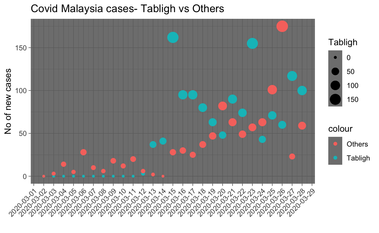
A few observations are in order:
- The first day of a large number of cases from the cluster is on 13th March, which is 12 days after the event.
- Cases related to the cluster kept coming in even until today (28th March), which is more than 25 days after the event.
Since the Tabligh cluster provides the single largest source of case data, it is pertinent that an investigation on this particular cluster is performed. This is the purpose of this writing.
Simulating dynamic ICM SIR model
First of all, let us model the overall process of disease transmission process from start-to-end, and how each compartment relates to each other, by modeling the relations and processes involved between all the compartments as described in the table below:
| Label | Compartment | Relations to | Direction |
|---|---|---|---|
| \(S\) | Susceptible | Exposed | \(S \to E\) |
| \(E\) | Exposed | Infected | \(E \to I\) |
| \(E\) | Exposed | Quarantine | \(E \to Q\) |
| \(I\) | Infected | Hospitalized | \(I \to H\) |
| \(Q\) | Quarantine | Hospitalized | \(Q \to H\) |
| \(Q\) | Quarantine | Recovered | \(Q \to R\) |
| \(H\) | Hospitalized | Recovered | \(H \to R\) |
| \(H\) | Hospitalized | Fatal | \(H \to F\) |
| \(R\) | Recovered | N/A | N/A |
| \(F\) | Fatal | N/A | N/A |
Network diagram
The diagram (flows) of ICM-SIR model is described in the following network plot:
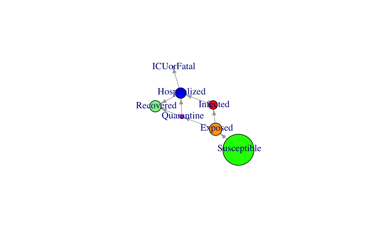
Note: Size of the network nodes is only indicative and do not reflect the actual numbers.
Model parameters assumptions
The dynamic ICM-SIR model is extremely sensitive to assumptions of various parameters used. Many simulations produced by various parties are produced for public consumption without detailing the assumptions used. As an example, a publication by JP Morgan recently published estimates that the total cases for Covid in Malaysia would reach more than 6,000 cases by mid-April, and another one by MIER (Malaysian Institute of Economic Research) says the figure could reach more than 8,000. Whilst all these modeling exercises have their own merits, we need to caution on a few concerns:
So far from our works, we have seen that models that relied heavily on \(R_o\) as the measure of outbreak growth rate would incur errors in estimations, mainly due to the variance in the \(R_o\) estimates. One of the major drawbacks is the lack of knowledge of modelers on the Serial-Interval distributions of Covid in Malaysia. So far, this has been much of guesswork at best.
In most of scientific publication, the publishers produced their estimates and allow the readers to understand their models - namely the type of models used (note that there is no proprietary model for Covid had been produced), key assumptions that they had made in regards to various model parameters, and importantly, the possible variations (upper bounds and lower bounds) of their estimates.
For our simulation of the ICM-SIR model, the assumption of the Serial-Interval distribution is from the family of discrete Weibull (an extended family of gamma distribution). Furthermore, we made many other assumptions that we try to mimic the possible situation of various issues at hand, such as “social distance”, heterogeneous interactions, delays in asymptomatic signs, as well as possibilities of infections before the asymptomatic stage, and many others. The parameters that we used for these assumptions are based on known parameters from other studies and situations. For example, we modeled that daily interaction between an infected person with susceptible persons to be in the range of 10 to 20 per day, as recorded in other studies.
Details of our model parameters and assumptions is enclosed in the appendix.
Tabligh cohort outbreak simulations
First, let us provide general statistical properties of our model in relations to a few major parameters estimated by our model and compare them with observed realities. Model plots are as attached below:
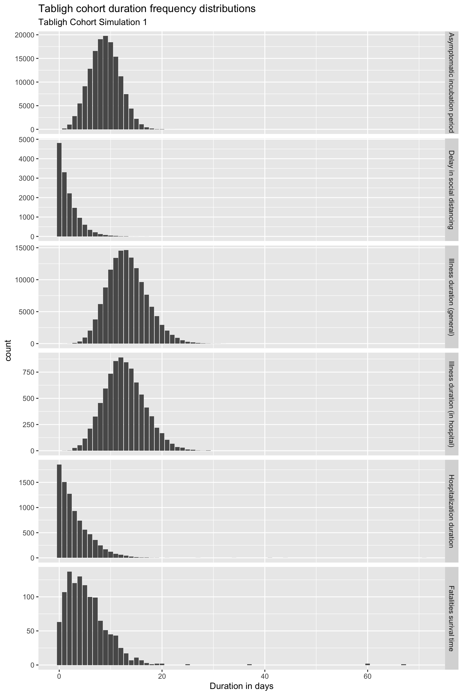
Comments:
- Asymptomatic incubation period - the median is about 10 days and some cases could reach 20 days or more. This is in confirmation with what we observe from the actual cases.
- Isolation started much later, could be as long as 10 days - many people took more than a few days before they started to isolate themselves because of being not aware of or due to some other reasons.
- Illness duration seems to match what’s observed.
- Hospital care duration also seems to match actual observations.
- Survival time of case fatalities is not known yet, hence it does not play a major role in our model.
Covid Tabligh cohort prevalence analysis
Now we want to study the disease prevalency of Covid outbreak based on model simulations. Prevalence is the number of count of people in each category (compartments on each day) as time progressed, as described by the ICM-SIR model described before.
The key questions that we want to understand are: how many of the 15,000 plus people who attended the gathering (Ijtima’) were potentially exposed to Case 136 person? And from these exposed people, how many would eventually contract the disease and how long before they all are hospitalized? This is presented in the plot of the disease prevalence among this cohort as shown below:
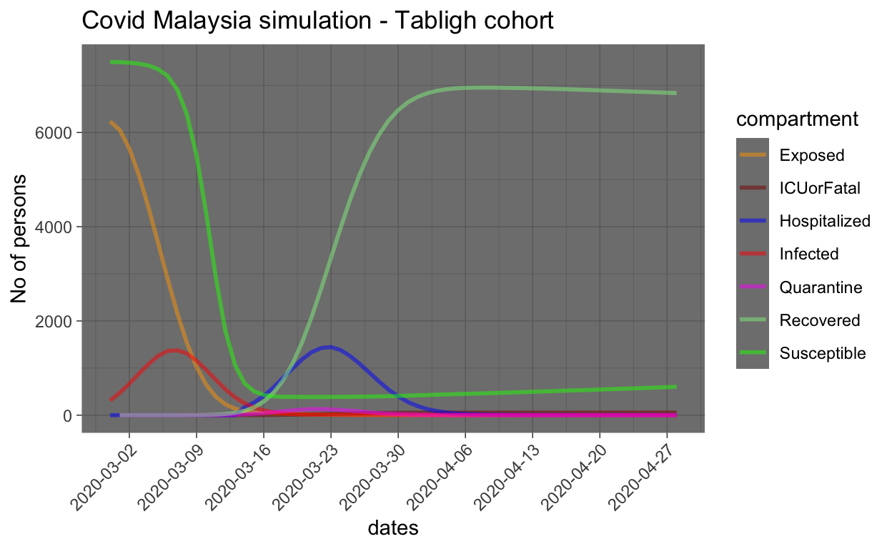
From the graph, the model estimate that from 15,000 susceptible people, about 6,000 people are potentially exposed during the 3 days event, and from this 6,000 plus, about 1,500 are potentially infected and require hospitalization. However, delays in the symptoms to show (as well as testing) and possible delays in the people getting to the hospital for checking, etc. causes about 15 days delay in the infected person to be hospitalized (and hence quarantined). Furthermore, the number of people who went to self-isolation is predicted to be small (based on the quarantine rate assumed in the model).
Generally, we can assume by now that most of the people from the Tabligh cluster had been tested, or if they are not tested and do not show any symptoms by now, they are either NOT exposed, or not infected (such as immunity). So the concerns about this cluster, as far as from primary infection (from Case 136) has significantly reduced (i.e. they have entered the Recovered group of the compartment, as shown in the graph (light green color)).
Now let us zoom into infected cases, hospitalization and ICU/fatalities.
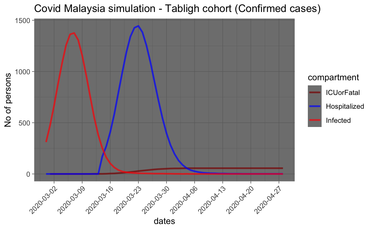
In order to make sense from the plot, we need to provide few notes of cautions:
- Since the records of the number of days of hospitalization are required by each patient is not publicly known, we can’t infer much from the simulation on how long the period would be. Furthermore, in the simulation, we do not provide much support for the parameters used due to this fact, and hence we may over/underestimate the duration of stay in the hospital (i.e. the recovery rate from infection).
- We also do not model the fatality rates meticulously since there are many unknown parameters involved, and hence estimates provided by the simulation are unreliable.
The model estimates that the peak number of infected people from the Tabligh cohort should be at about 1,500 people and the peak is about now. By now, most of confirmed cases should have been identified and hence hospitalized.
What could we learn and the next step
If the estimates of the simulation as provided above are reflective of the reality, then it raises many other questions about the overall epidemics:
- How much do these Tabligh infected cohorts spread the disease while they are NOT yet quarantined or hospitalized(i.e. they are infected and infectious), especially during the period of between 1 to 14 days (approximately) while they are mixing in the open (at least until 18 March onwards)? (i.e. secondary infection)
- How about other sources of infection, which are not from the Tabligh cohort?
- Do the third level or higher level of infection occurs? As commented by DG of Health, from the Tabligh cohorts, there is evidence that even the fifth level exists.
To simulate the overall picture of the country, then we need to develop a more comprehensive model. Which we will turn to in the next article.
Excerpt from the latest news
News on 27 March: From the Tabligh Cohort, 711 index cases had infected their families (first generation), and possibly five generations exist. The Tabligh Cohort made up 55% of all cases in the country - 1,117 from 2031. A total of 13,762 Tabligh attendees were screened with 9,327 samples taken to be tested of which 1,117 of the samples tested positive, a total of 5,646 were negative while 2,564 were still pending for the result.
On March 28 DG MOH reports that: 12,500 attendees samples tested, 1,207 tested positive and 6,648 negatives, while 4,645 others pending. 5,804 have not been tested (or found). On secondary cases emanating from Tabligh cluster, 4 clusters are believed to occur in two villages in Simpang Renggam, Johor.
Conclude
Based on what we simulate here, the number of cases from the Tabligh Cluster should peak to about 1,500 people, where most of the cases would have been confirmed by about these few days. If this is true, then more focus and concern should be on secondary or tertiary transmission induced by the original cohort, and other non-clustered cases.
Model simulation parameters
We will now provide the various assumptions required for creating a simulation for the base model:
Simulation and computation settings:
| Parameters | Choice | Notes |
|---|---|---|
| type | “SEIQHRF” | describes the compartment network that we have chosen |
| nsteps | 365 + 1 | days for a year + 1 |
| nsims | 20 | number of times to run simulations |
| ncores | 12 | cores used for parallel computing |
| out | “mean” | choices of “mean”,“median”, “quartiles” as simulation output |
Probability and distributions settings:3
| Parameters | Value | Notes |
|---|---|---|
| Infections | ||
| prog.rand | FALSE | \(E \to I \sim\) discrete Weibull distribution for infection |
| prog.dist.shape | 2.5 | \(\alpha\) shape of the curve (rate of infections) |
| prog.dist.scale | 15 | \(\beta\) scale of the curve (uration of infections) |
| prog.rate | 10/100 | rate/day Exposed people become asymptomatic (Infected) |
| Recovery | ||
| rec.rand | FALSE | \(H \to R, Q \to R \sim\) discrete Weibull distribution for recovery |
| rec.dist.shape | 1.5 | \(\alpha\) shape of the curve (rate of recovery) |
| rec.dist.scale | 35 | \(\beta\) scale of the curve (duration of recovery) |
| rec.rate | 2/100 | rate/day Infected people recovered |
| Fatalities | ||
| fat.rand | FALSE | \(H \to F \sim\) random sample from \(fat.rate.base\) distribution |
| fat.rate.base | 1.5/100 | rate of fatality from hospitalized cases |
| fat.rate.overcap | 1/1000 | rate of fatality due to can’t get hospitalization |
| fat.tcoeff | 0.2 | linear scale increase of mortality as time of hosp. increase |
| Quarantine | ||
| quar.rand | FALSE | \(I \to Q \sim\) random sample from \(quar.rate\) distribution |
| quar.rate | 1/30 | rate/day Exposed enters Quarantine |
| Hospitalization | ||
| hosp.cap | 2/1000xN | hospital max capacity for the population \(=(2/1000)*pop\) |
| hosp.rand | FALSE | \(I \to H, Q \to H \sim\) random sample from \(hosp.rate\) distribution |
| hosp.rate | 30/100 | rate/day Infected enters Hospitalization |
| disch.rand | FALSE | \(H \to R \sim\) random sample from \(disch.rate\) distribution |
| disch.rate | 2/100 | rate/day Hospitalized are discharged (i.e.Recovered) |
Initial parameters settings:
| Parameters | Value | Notes |
|---|---|---|
| \(i.num\) | 1 | Number of Infected person at the onset |
| \(s.num\) | 15000 - 1 | Number of Susceptible at the start |
| \(e.num\) | 0 | Number of Exposed at the onset |
| \(q.num\) | 0 | Number of Quarantined at the onset |
| \(h.num\) | 0 | Number of Hospitalized (Covid) the onset |
| \(r.num\) | 0 | Number of Recovered at the onset |
| \(f.num\) | 0 | Number of Fatal at the onset |
| \(inf.prob.i\) | 0.15 | Probability of infection on Susceptible people based on interactions with orginally infected (I) people, \(i.num\) under each exposure event, called \(act\) |
| \(act.rate.i\) | 20 | Number of \(act\) between infected person and susceptible person per day, which may results in infection based \(inf.prob.i\) rate |
| \(inf.prob.e\) | 0.10 | Probability of infection on Susceptible people based on interactions with exposed people (E), \(i.num\) under each exposure event, called \(act\) |
| \(act.rate.e\) | 10 | Number of \(act\) between exposed person and susceptible person per day, which may results in infection based \(inf.prob.e\) rate |
| \(inf.prob.q\) | 0.05 | Probability of infection on Susceptible people based on interactions with quarantined (Q) people, \(i.num\) under each exposure event, called \(act\) |
| \(act.rate.q\) | 2 | Number of \(act\) between infected person and susceptible person per day, which may results in infection based \(inf.prob.q\) rate |
Function settings:
| Functions | Choice | Notes |
|---|---|---|
| infection.FUN | infection.seiqhrf.icm | Function for infection process used in the model |
| departures.FUN | departures.seiqhrf.icm | Not applicable (since vital = FALSE) |
| arrivals.FUN | arrivals.icm | Not applicable (since vital = FALSE) |
| get_prev.FUN | get_prev.seiqhrf.icm | To carry recursive results in the simulations |
Demographic movement parameter settings:
| Parameters | Value | Notes |
|---|---|---|
| vital | FALSE | Do not allow changes in demographic to take place (in the model) |
| a.rates, etc. | N/A | All rates related to demographic changes dynamics |
Jennes, S.M., Goodreau, S.M., Morris, M., EpiModel: An R Package for Mathematical Modeling of Infectious Disease over Networks, Journal of Statistical Software, April 2018, Volume 84, Issue 8. https://doi.10.18637/jss.v084.108↩
https://github.com/timchurches/blog/tree/master/_posts/2020-03-18-modelling-the-effects-of-public-health-interventions-on-covid-19-transmission-part-2↩
A short note on Weibull distribution: “shape” (\(\alpha\)) control the “heights” of the curve, while, “scale” (\(\beta\)) control the “dispersion” of the curve. Since we assume that \(\alpha > 1\) and \(\beta > 1\), the curve will have a peak, with slopes on left and right of the peak. Mean \(= \beta*\Gamma(1 + \frac{1}{\alpha})\). For example, if \(\alpha = 2\) and \(\beta = 5\), \(mean = 5*\Gamma(1 + \frac{1}{2}) = 4.43\). It means that the mean for the period of infection is at 4.43 days. Hazard rate, or \(R_o\) is \(= \alpha*\beta^{-\alpha}*t^{\alpha-1}\).↩