Table of Contents
Pre-amble
Most of epidemic modeling uses some forms of SI models, such as SIR, SIRS, and others. In this article, we present a simplified analysis of SIR model (which is assumed to be applicable for Covid). SIR model assumes that the disease is spread from Infectious person to Susceptible person at a certain rate (or process). It models how the disease could spread and hence generate epidemics to the population at large. Covid in Malaysia, as of today is confirmed as an epidemic of a scale that is unprecedented in our history (and globally in human history). As such, it is rather pertinent that we use data science tools to study and understand this phenomenon better. This is the purpose of this article and a few other subsequent articles that we will publish. Tracking and understanding Covid as it progress provides many insights about human and human behaviors at large.
Some of the codes are obtained from Tim Churches1, as well we use packages from R Epidemics Consortium (RECON)2, and our codes developed by Techna Analytics Sdn. Bhd. In particular, we rely on the following packages in R: distcrete, epitrix,incidence,earlyR, and most notably EpiEstim.
Malaysian covid situation
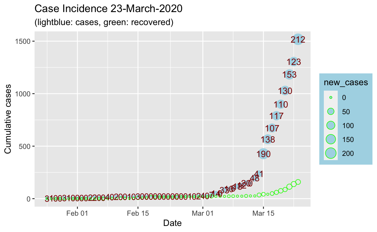
First and foremost, let us summarize the data on Malaysian Covid outbreak, from publicly available data. For this purpose, we will use “line data” as provided by John Hopkins University which had taken the efforts to compile all Covid data globally and updated daily. The data source is from the John Hopkins database3 and Techna Analytics own compiled data from publicly available official information (Malaysian Ministry of Health announcements).
Let us summarize the stats obtained from the data:
Comments on analysis and methods
By the time of this writing, COVID-19 is already a global pandemic. The question is could Malaysia learn from data available from other countries as well as lessons to be learned from their efforts, as well as our local efforts?
Critical to this exercise is learning by using models, rather than pure conjecture and speculations. Why models? It is the standardized methods used by health authorities worldwide; it allows sharing of methodologies and findings systematically; it’s done as reproducible research and sharing of findings, which means allows validations by other parties in a transparent manner and permeation of knowledge and learning; and so on.
An important element of modeling is the programming language used, of particular focus is on Open Source languages, and of interest here is R Programming Language. Epidemics modeling requires extensive mathematical modeling and statistical computations for which SAS, SPSS, Matlab, Stata, are among the languages that had performed well and are widely in used by biostatisticians. R is a recent entrant into this field - albeit as an open-source. The advantage of R is that it is a programming language and hence the flexibility of altering and modifying codes, which allows greater latitude when it comes to modeling and becomes a handy tool for modeler (as opposed to running ready-made models). The biggest advantage of R is the contributions to package developments - and in particular, in regards to epidemics, it has one of the largest developments among all open source languages. Here we will rely heavily on R packages developed and published by the R Epidemics Consortium (RECON).
Basic SIR model
Basic SIR model assumes: Susceptible persons \(\to\) Infected persons \(\to\) Recovered persons (or Fatal).
\[S_t \to I_t \to R_t\]
The process of transitions from S to I and to R is represented in the following ordinary differential equations (ODEs) as follows:
\[\frac{\delta S}{\delta t} = - \beta * \frac{I*S}{N} \ \ Equation \ 1\]
\[\frac{\delta I}{\delta t} = \beta * \frac{I*S}{N} - \gamma*I \ \ Equation \ 2\]
\[\frac{\delta R}{\delta t} = - \beta * \frac{I*S}{N} \ \ Equation \ 3\]
where: \(\beta\) and \(\gamma\) are the control operators of the transitions between \(S \to I\) and \(I \to R\) respectively.
To estimate \(\beta\) and \(\gamma\), we need to perform parameters estimations using Residual Sums of Squares on the ODEs: \[RSS(\beta,\gamma) = \sum_{t}(I_t - \hat{I_t})^2\]
To calculate \(R_o\) we use:
\[R_o = \frac{\beta}{\gamma}\]The following table presents \(R_o\) for various countries based various dates for the early days of the epidemic:
| Country | Start Date | End Date | Population | \(R_o\) estimate |
|---|---|---|---|---|
| Malaysia | “2020-02-04” | “2020-03-23” | 30 million | 1.1702429 |
| Italy | “2020-02-04” | “2020-03-15” | 70 million | 1.5668066 |
| Singapore | “2020-02-04” | “2020-03-15” | 6 million | 1.1182783 |
| Thailand | “2020-02-04” | “2020-03-15” | 70 million | 1.0529511 |
| Philippines | “2020-02-04” | “2020-03-15” | 100 million | 1.2001347 |
| Vietnam | “2020-02-04” | “2020-03-15” | 90 million | 1.0848888 |
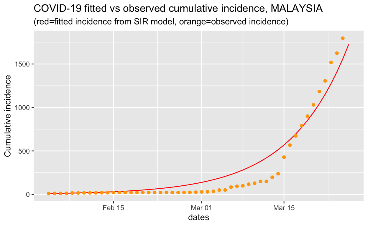
We can see that from the plot, it is showing that the \(R_o\) estimates capture the growth of the outbreak closely. The defect of the approach, however, is that it is highly dependent on the choice of starting and ending date.
Modelling growth rate using log-linear models
Another approach of modelling is to use simple log-linear growth and decay function of the form:
\[log(y) = rt + b\] where \(y\) is the incidence, \(r\) is the growth rate, \(t\) is days since start of outbreak, and \(b\) is the intercept.
First, let us try to get a better hold of the growth parameters of the Malaysian Covid case by running a log-linear estimation and analyze the results.
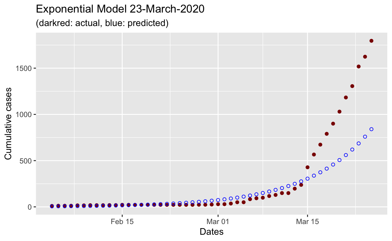
We can see that the exponential model underestimates the actual growth of the outbreak.
Before proceeding further, let us try to understand the behavior of \(R_o\) based on the estimates obtained. It is generally assumed that \(R_o\) follows a gamma distribution, hence we will try to observe the shape of the distribution of \(R_o\) from the model obtained above.
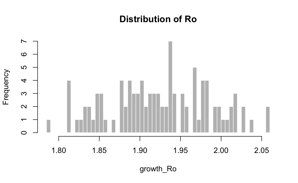
   Min. 1st Qu.  Median    Mean 3rd Qu.    Max.
  1.786   1.883   1.924   1.924   1.971   2.060
It is evident that estimating \(R_o\) using an exponential curve such as gamma distributions doesn’t fare too well in the Covid case for Malaysia. This called for a better way to estimate \(R_o\) as it progresses on a daily basis.
Estimating reproduction (\(R\)) rate on a daily basis
To see the growth of the outbreak on a daily basis, we need to obtain estimates of Ro for each day as the outbreak progressed. This measure is called \(R_e\).
We will focus on one method, developed in 2013 by Anne Cori and colleagues at Imperial College, London, which permits estimation of the instantaneous effective reproduction number, which is required for tracking the effectiveness of containment efforts. This is achieved through EpiEstim package in R.
Let’s make some observations:
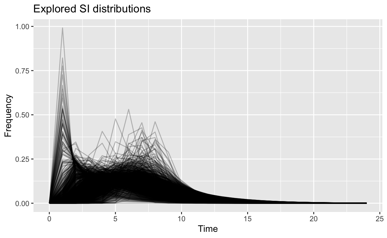
Using observations of estimates for the gamma distributions (ranges of the mean and standard deviation) from other countries helped us to generate more robust estimates of \(R_o\) and \(R_E\) for Malaysian case, which is presented by the plots.
The first plot, which shows the distribution of the Serial-Interval (SI) for Covid in Malaysia shows that the intervals between cases (from the date of infection till being confirmed) varies largely between 1 to 10 days, and even maybe as long as 20 or more days. This is the measure of what is called the generation period for the disease. This is an important parameter to be taken into consideration for further modeling.
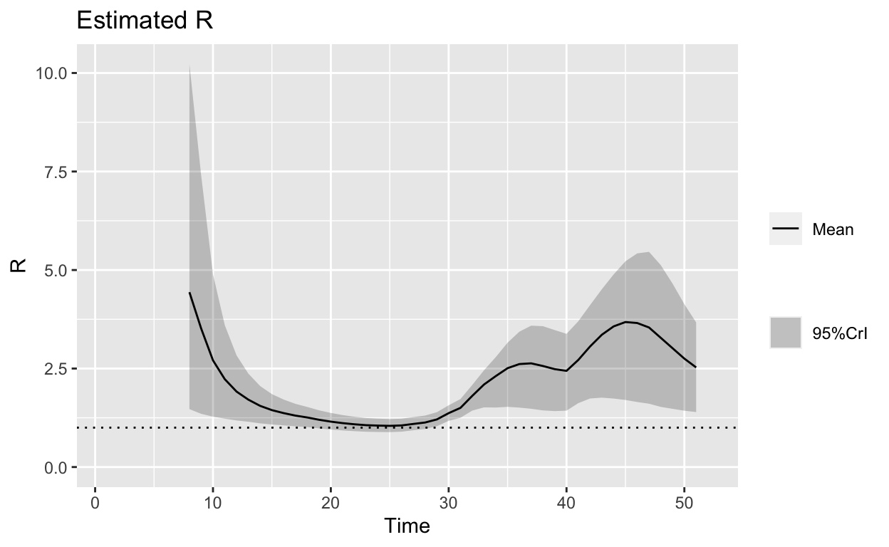
- The second plot, which shows the possible ranges of \(R_o\) over the days as the outbreak occurs reveals few important points:
- At the beginning of the outbreak, \(R_o\) was high (mean of about 5, and a maximum of 10), which explains the high speed of the outbreak at the early stages.
- More importantly, the \(R_o\) measure increases again after 30 days, which could happen by several reasons: a) the delayed time for the disease to show its symptoms (hence delayed confirmation), or b) there are new cases that came into the picture. Without further details, it is very hard to separate these two reasons.
- In any case, the \(R_E\) measures as of March 23 (Time = 50) is still very high (mean of about 2.5) with large variations (maximum of 4 and minimum of 1.5). Again, we can’t be sure whether this is due from new cases of infection or due to delay in confirmation as mentioned in (ii) above.
Conclude
We have shown in this writing how rudimentary methods of calculating \(R_o\) (or \(R_E\)) are prone to too many errors in the estimates and hence unreliable to be used for policymaking tools. Hence a more dynamic approach (as suggested by the methodology proposed by Imperial College) is pertinent in measuring the Covid outbreak as it progresses.
In the next article, we will address more comprehensive modeling of the outbreak and how we could use the results for predictions and policymaking exercises.